Isaias will be the ninth tropical storm of the season, likely to form on July 30. This is unusually early. From CNN on July 28: “Once it is given the name Isaias — pronounced (ees-ah-EE-as) — it will be the earliest storm to begin with an “I” on record. The previous record was set on August 7, 2005, part of the busiest season to date.”  Storms are named in alphabetical order, so a storm starting with “I”  is the ninth storm of the season.

This did seem early to me. The recent example that I remember Irma, which made landfall on the mainland US on September 10, 2017. (I spent a day seeing lots of people with Florida license plates driving around Atlanta, thinking “at least I don’t live in Florida!”, and then the next day having my power out and being glad that the trees the storm took out in my backyard were ones that needed taking out anyway.)

What does this mean for the rest of the hurricane season? Should we expect a busy one?

There’s an R package, HURDAT, that compiles the NOAA hurricane database. For each year, we can count the number of storms. First let’s make a list of all the storms:

library(HURDAT)
library(lubridate)
al <- get_hurdat(basin = 'AL') cutoff_month = 7 cutoff_day = 29 storms = al %>% group_by(Key) %>% filter(Status %in% c('TS', 'HU')) %>%
mutate(rk = rank(DateTime)) %>% filter(rk == 1) %>%
mutate(season_part = ifelse(month(DateTime) < cutoff_month |
month(DateTime) == cutoff_month & day(DateTime) <= cutoff_day, 'early', 'late')) %>%
select(Key, Name, DateTime)


and count the storms by time in the season:

storm_counts = storms %>% mutate(yr = year(DateTime)) %>%
group_by(yr, season_part) %>% count()

But how do we know about are storms? Not all storms were observed in the past, because some stay out to sea. The “satellite era” began in 1966, according to this article about this year’s Tropical Storm Gonzalo (the earliest “G” storm ever). So let’s plot the number of storms before and after July 29, separately for each of the two “eras”.

satellite_start = 1966
storm_counts %>% spread(season_part, n, 0) %>%
mutate(satellite = ifelse(yr >= satellite_start, 'satellite', 'pre-satellite')) %>%
ggplot() + facet_wrap(~satellite) + geom_jitter(aes(x=early, y=late)) +
stat_smooth(aes(x=early, y=late, group = satellite), method = 'lm') +
scale_x_continuous(paste0('storms before ', cutoff_month, '/', cutoff_day)) +
scale_y_continuous(paste0('storms after ', cutoff_month, '/', cutoff_day))


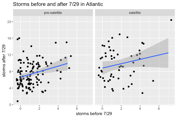
But 2005 is a big outlier! I remember that season. Of course it was the year of Katrina. And in December there was a hurricane named Epsilon, which I could not take seriously because epsilon is small. Indeed if we drop it the effect of early-season storms on late-season ones gets much smaller.

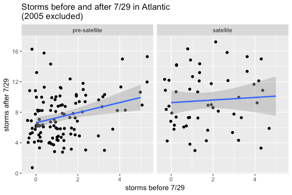
So there’s a small effect – but not as large as might be expected! So how many storms will we have this season? Calling predict(storm_model, data.frame(early = 9), interval = 'prediction', level = 0.95), gets a 95% prediction interval for the number of storms in the rest of the season: 12.5 plus or minus 7.2. So we could reasonably have as few as 5 more or as many as 20 more, for a total of 14 to 29.

A 50% prediction interval goes from 10 to 15 more storms in the remaining part of the season, for a total of 19 to 24. For comparison, the quartiles of the distribution of the number of storms after 7/29 in the satellite era are 7 and 12. So if we knew nothing about what’s happened so far, we’d give a 50% prediction interval of 16 to 21 storms for the number at the end of the season.

Let’s see what happens. And let’s hope these storms stay far out to sea, because pandemics and hurricanes don’t seem very compatible.

Here’s a sequence I keep mulling over in my head:

1, 2, 4, 8, 16, 23, 46, 29, 58, 116, 223, 446, …

Does it grow without bound? First we should specify what it is. Each number is double the one before, but with the digits sorted into ascending order. The doubling makes the number larger… but the sorting makes it smaller, so perhaps this sequence tops out somewhere?

This sequence actually becomes periodic pretty quickly. The full sequence is:

1, 2, 4, 8, 16, 23, 46, 29, 58, 116, 223, 446, 289, 578, 1156, 1223, 2446, 2489, 4789, 5789, 11578, 12356, 12247, 24449, 48889, 77789, 155578, 111356, 122227, 244445, 48889, …
and then it repeats with period 6. The key is in the final step: once we get a number that ends with 5, there’s a 0 in its double so the next term is actually shorter. (It is surprisingly hard to keep the mental arithmetic straight to the point where I can do this in my head.) There are other such loops: if you start with 3 you eventually reach

69, 138, 267, 345, 69, …

(note that everything stays divisible by 3 here!). If you start with 7 you get to

167, 334, 668, 1336, 2267, 3445, 689, 1378, 2567, 1345, 269, 358, 167, …

and if you start with 9 you get to

9, 18, 36, 27, 45, 9, …

And there’s a series of these sequences. Every number in that period-6 loop that you reach if you start with 1 has a repeated digit, and you can have less or more of those:

49, 89, 178, 356, 127, 245, 49, …
489, 789, 1578, 1356, 1227, 2445, 489, …
4889, 7789, 15578, 11356, 12227, 24445, 4889, …

The structure is quite a bit richer than the triple-and-sort sequence, presumably because divisibility by three “plays well” with rearranging digits. There, as far as I can tell, no matter what number you start with you end up with 45. (Tripling that give 135, tripling again gives 405, which sorts back to 45.) The reason for this seems to be that any repeated digits, when tripled, give you repeated 3s or 6s, and tripling those gives repeated 0s. For example, consider the start number 9261632697:

• Tripling gives 27784898091 – which incidentally has a zero – and sorting that gives 1247788899.
• Tripling again gives 3743366697 – the repeated 7s and 8s “turn into” repeated 3s and 6s — and sorting gives 3334666779.
• At this point everything collapses – tripling gives 10004000337, and sorting gives 13347.
• Another collapsing step: 13347 × 3 = 40041, which sorts to 144.
• The remainder of the sequence is uninteresting:  234, 27, 18, 45, 135, 45, 135, …

This is the “typical” behavior – but it’s a bit surprising to me that it always works. I suspect a proof would be in terms of vectors that show the number of each digit, rather than with the raw numbers themselves.

Riddler Express for July 3, 2020:

Suppose a queue of swimmers arrives at [a] pool when it opens at 9 a.m. One at a time, each person randomly picks a lane from among the lanes that are available (i.e., the lane has no swimmer already and is not adjacent to any lanes with swimmers), until no more lanes are available.

At this point, what is the expected number of swimmers in the pool?

For five lanes the pool will be full when lanes 1, 3, and 5; 1 and 4; or 2 and 5 are occupied.

If lane 2 is first to be filled then we will certainly end up with just two occupied lanes (2 and 4); similarly with 4.

If lane 3 is first we certainly end up with three occupied lanes, since 1 and 5 remain and they don’t interfere with each other.

If the first swimmer uses lane 1 we actually have to think. The remaining lanes are 3, 4, and 5. If the second swimmer fills one of the “new” edge lanes (3 or 5) first then we’ll end up with three full lanes; if the second swimmer fills up 4 we end up with two full lanes. So if the first swimmer fills lane 1 we have an expectation of 2 2/3 lanes full, and similarly for lane 5.

Putting it all together the expected number of full lanes is .

This is sort of a discrete version of “Renyi’s parking problem”: if you have a street of length x and cars of length 1 park at random, how full is the street expected to be when nobody else can park?

In the n-lane case there’s a recursive solution. Let f(n) be the expected number of full lanes in an n-lane pool. Clearly f(1) = 1, f(2) = 1; we already worked out f(5) = 8/3.

To find f(n), consider where the first swimmer goes.

• If they use lane 1 or lane n then there is one remaining sub-pool of n-2 lanes.
• If they use lane 2 or lane n-1 then there is one remaining sub-pool of n-3 lanes.
• If they use lane with then there are two remaining sub-pools of k-2 and n-k-1 lanes.

So this gives us, if ,
$
with the base cases f(1) = 1, f(2) = 1, f(3) = 5/3.

If we compute this for large n we get , which agrees with the Monte Carlo simulations in Georgiou, Kranakis, and Krizanc 2009. (Simulation isn’t necessary here but it’s necessary if you consider an analogous problem on a grid.) The constant is . Kranakis and Krizanc have some online notes on the urinal problem. as well, and the problem goes back at least to a problem posed in the SIAM Review in 1962 by Freedman and Shepp.

(2020-07-07: fixed numerical expression of constant 0.4323)