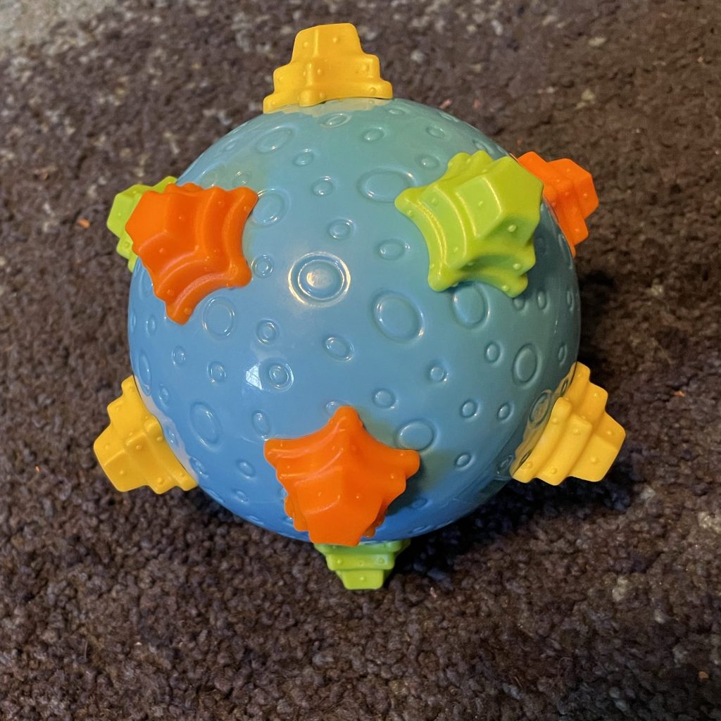
Somehow toys just show up in this house, a phenomenon which I think is familiar to many parents. Some of them have icosahedral symmetry. Like this one.
Hard plastic icosahedron ball, with stars for vertices.
You can see that the designer was outlining the vertex of an icosahedron with that five-pointed star shape, but they couldn’t quite commit – the star points don’t actually point to the next vertex! (And no, they don’t turn.) You can get a better sense of the stars corresponding to the vertices of an icosahedron here:
There’s also this one, which is softer and has a couple of distinguished vertices antipodal to each other:
Soft icosahedron, with rattly bits at two antipodal vertices.
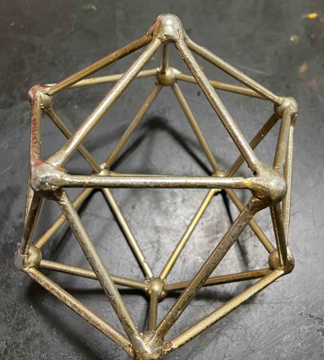
And this one which I bought for myself years ago, presumably in some sort of store that sold housewares. (Remember stores?)
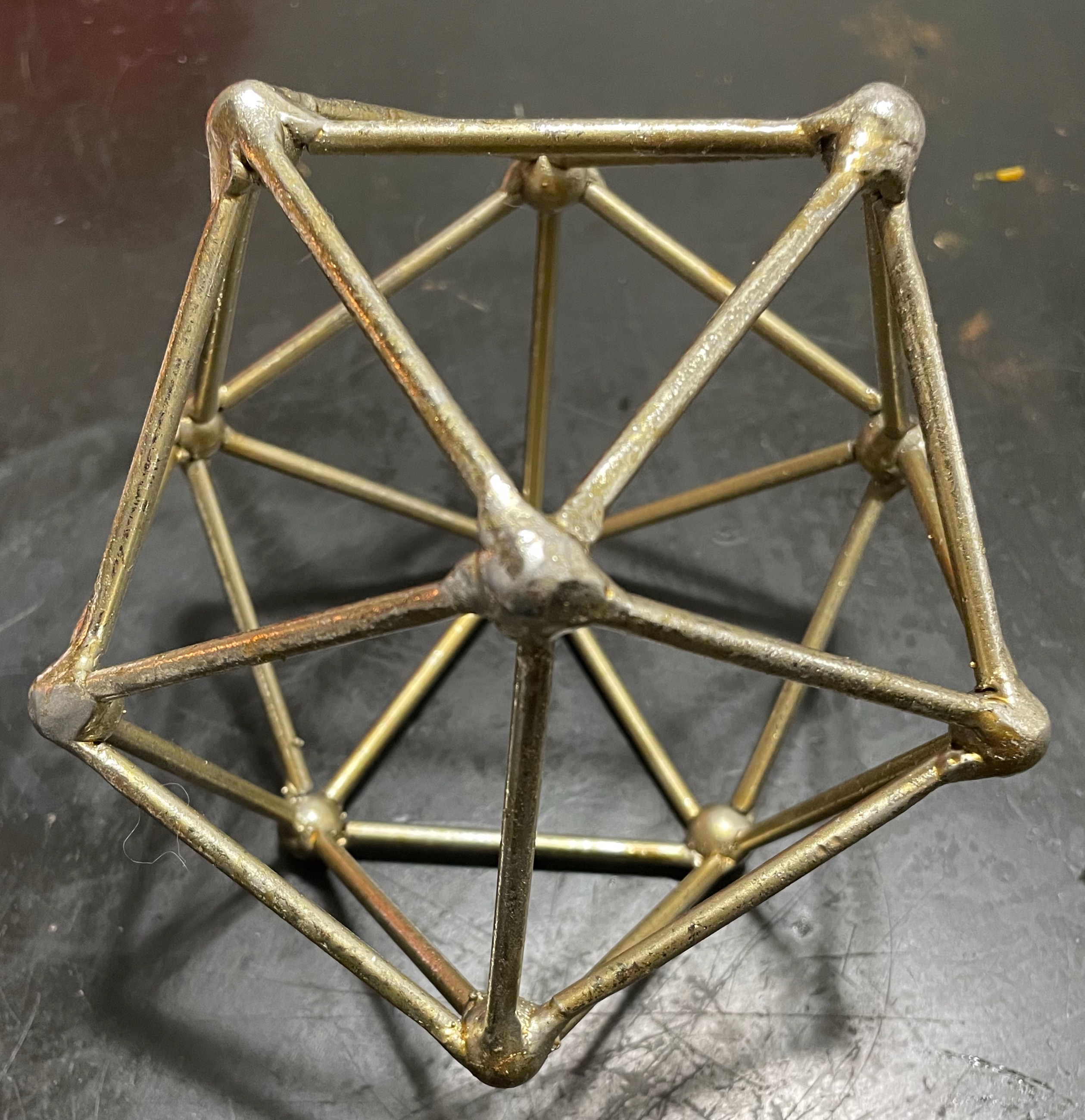
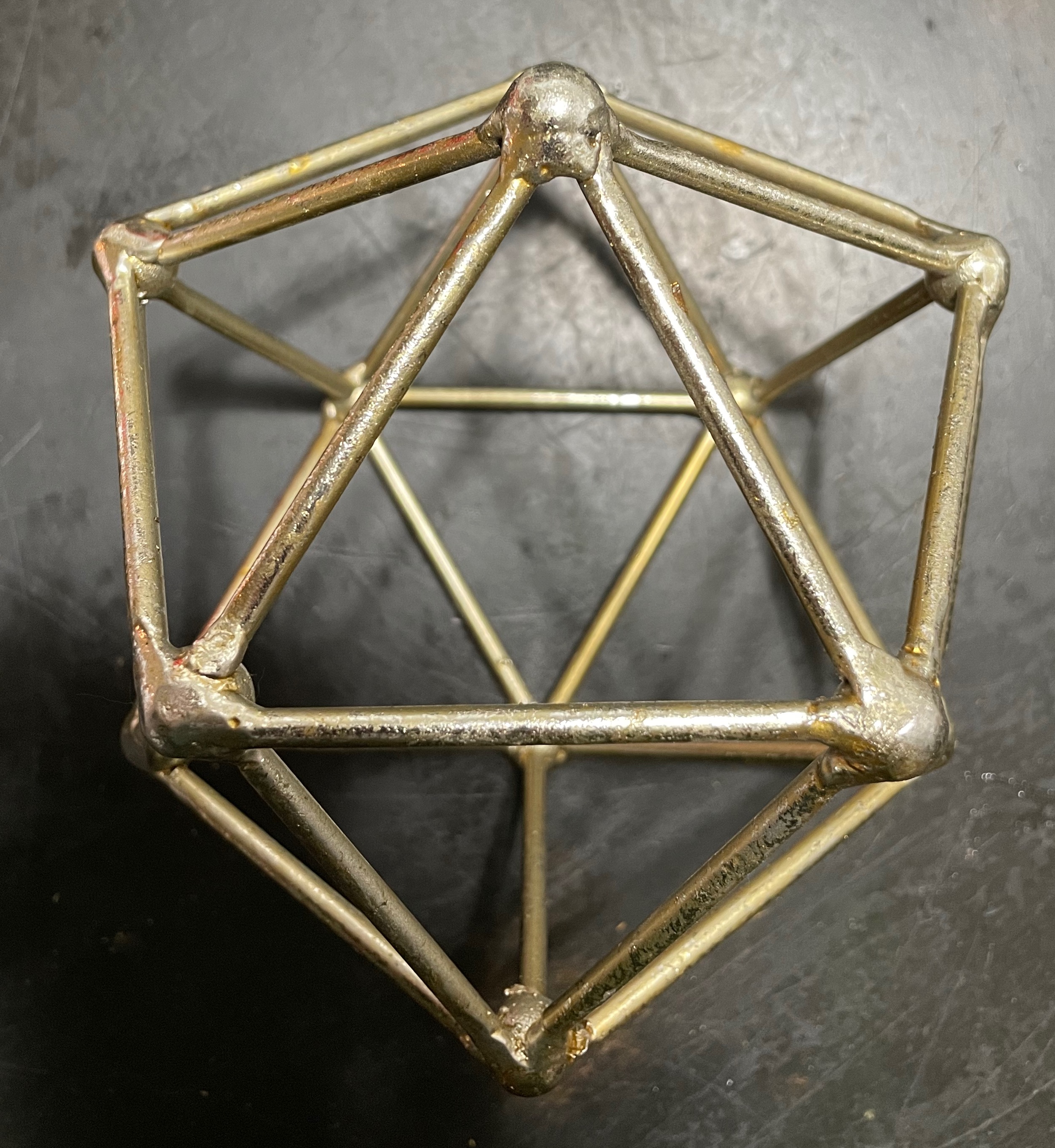
Skeleton of an icosahedron.
The nice thing about this one is that you can see through it, which makes for some interesting photographic possibilities, such as this view where two antipodal vertices are aligned:
Skeleton of an icosahedron, photographed down an axis through two vertices.
and this view with that emphasizes a threefold rotational symmetry:
Skeleton of an icosahedron, emphasizing threefold symmetry.
Of course we have a soccer ball somewhere. You know what a soccer ball looks like, I’m not taking a picture.
I also use this as an avatar in various work systems that need one – these generally require small pictures and a face wouldn’t show up well, and it’s easier to pick out than the default in a lot of these systems which is just someone’s initials in a circle.
I had thought, for a few decades now, that STOP was the four-letter word with the most anagrams, with six: STOP itself, POST, POTS, TOPS, OPTS, SPOT. So of course when Josh Millard put out these STOP permutations signs, I had to buy one. It’s a limited edition of 24 stop sign prints, one for each permutation. (I opted for OPTS. As of this writing there are 18 still available; the 6 that have been bought are the five anagrams of STOP other than STOP itself, and SOTP.)
But then I had to check that claim. Peter Norvig has, meant to accompany a chapter on NLP, some word lists, of which I’ve used the enable1.txt list before for word puzzles. (I’m not sure who compiled this list.) We can put words into a canonical form by alphabetizing the letters – for example michael becomes acehilm, and stop becomes opst. Scrabble players call this an alphagram. Then to find the four-letter word with the most anagrams is just a matter of counting.
But wait! What is “seta”? Is “ates” really a thing – you can’t pluralize a verb like that! (“ate” appears to be Tagalog for “older sister”.) Perhaps the aers set, with seven anagrams, wins, but “sera” is technical (plural of serum), and as an American I have trouble recognizing “rase” as a legitimate spelling of “raze”. “lari” is a unit of money in Georgia (Tbilisi, not Atlanta) which I was unfamiliar with. And so on.
Fortunately Norvig also has a list of word frequencies (count_1w.txt), of the 332,202 most common words in a trillion-word corpus. (One of the perks of working at Google, I assume.) So we can read that in.
The most common words are the ones you’d expect. (2.3% of words are “the”.)
> head(freqs)
# A tibble: 6 x 2
  word         freq
  <chr>       <dbl>
1 the   23135851162
2 of    13151942776
3 and   12997637966
4 to    12136980858
5 a      9081174698
6 in     8469404971
And the least common words are… barely words. (I don’t know the full story behind this dataset.) So it seems reasonable that all “real” words will be here.
> tail(freqs)
# A tibble: 6 x 2
  word     freq
  <chr>   <dbl>
1 goofel  12711
2 gooek   12711
3 gooddg  12711
4 gooblle 12711
5 gollgo  12711
6 golgw   12711
Now we can attach frequencies to the words. There are too many words in the sets for a table to be nice, so we switch to plots.
words %>% left_join(alphagram_counts)  %>%
  filter(len ==  4 & n >= 6)  %>%
  left_join(freqs) %>% arrange(alphagram, desc(freq)) %>%
  select(alphagram,  word, freq) %>% group_by(alphagram) %>%
  mutate(rk = rank(desc(freq))) %>%
  ggplot() + geom_line(aes(x=rk,  y=log(freq/10^12, 10), group = alphagram, color = alphagram)) +
  scale_x_continuous('rank within alphagram set', breaks  = 1:8, minor_breaks = c()) +
  scale_y_continuous('log_10 of word frequency', breaks = -8:-3, minor_breaks  = c()) +
  theme_minimal() + geom_text(aes(x=rk, y=log(freq/10^12, 10), color = alphagram, label = word)) +
  ggtitle('Frequency of four-letter words with six or more anagrams')
And if we plot the frequency of each word against its rank in its own anagram set…
then we can see that the STOP set consists of much more common words than any of the others. (STOP isn’t even the most common of its own anagrams, which surprises me – that honor goes to POST. But when I was a small child STOP seemed much more common, because of the signs.) I’m surprised to see SERA so high; this is either an extremely technical corpus or (more likely) contamination from Spanish.
And here’s a similar plot for five letters. Here I’d thought the word with the most anagrams was LEAST (among “common” words, 6: TALES, STEAL, SLATE, TESLA, STALE) but it looks like SPARE wins with room to spare, even if you don’t buy that APRES is an English word.


