John Cook, at his Probability Fact twitter feed (@ProbFact), asked (I’ve cleaned up the notation):
What is the expected amplitude for the sum of  sines with random phase? i.e. sum of
  where
where ![\phi_i ~ uniform[0, 2\pi]](https://s0.wp.com/latex.php?latex=%5Cphi_i+%7E+uniform%5B0%2C+2%5Cpi%5D&bg=ffffff&fg=000000&s=0&c=20201002)
Intuitively one expects something on the order of  , since we’re adding together what are essentially independent random variables. It’s not too hard to throw together a quick simulation, without even bothering with any trigonometry, and this was my first impulse. This code just picks the
  uniformly at random, and takes the maximum of
 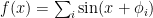 for values of
  which are multiples of
  .
.
x = (0:200)/(2*Pi)

n = 1:100

num.samples = 100
max.of.sines = function(phi){

max(rowSums(outer(x, phi, function(x,y){sin(x+y)})))

}
mean.of.max = function(n, k){mean(replicate(k, max.of.sines(runif(n, 0, 2*pi))))}

averages = sapply(n, function(n){mean.of.max(n, num.samples)})
This is a bit tricky: in the matrix in max.of.sines, output by outer, each column gives the values of a single sine function , and rowSums adds them together.
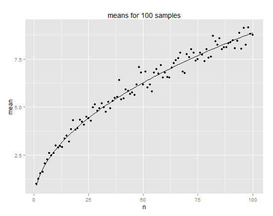
We can then plot the resulting averages and fit a model  . I get
  from my simulation, which is close enough to
  to ring a bell:
C = lm(averages^2~n+0)$coefficients
qplot(n, averages, xlab="n", ylab="mean", main="means for 100 samples") +

stat_function(fun = function(x){sqrt(C*x)})

At this point we start thinking theory. If you’re me and you haven’t looked at a trig function in a while, you start at the wikipedia page, and discover that it actually does all the work for you:

where
 .
.
That is, the sum of a bunch of sinusoids with a period is a single sinusoid with the same period, and an amplitude easily calculated from the amplitudes and phases of the original sinusoids. There’s a formula for  as well, but it’s not relevant here.
In our case all the  are 1 and so we get
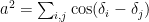
If you take the expectation of both sides, and recognize that  is 1 if
  (it’s
(it’s  ) and 0 if
  (just the average of the cosine function), then you learn
  where is the number of summands. That agrees with our original guess, and is enough to prove that
  by Jensen’s inequality.
To get the exact value of  we can expand on David Radcliffe’s comment: “Same as mean dist from origin after N unit steps in random directions. Agree with sqrt(N*pi/4)”. In particular, consider a random walk in the complex plane, where the steps are given by
  where
where  is uniform on the interval
  . We can work out that its sum after steps is

and so, breaking up into the real and imaginary components,
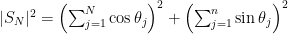 .
.
Rewriting the squared sums as double sums gives

and combining the double sums gives

and by the formula for the cosine of a difference we get

which is exactly the  given above. So the amplitude of our sum of cosines is just the distance from the origin in a two-dimensional random walk!
It just remains to show that the expected distance from the origin of the random walk with unit steps in random directions after steps is  . A good heuristic demonstration is as follows: clearly the distribution of the position
  is rotationally invariant, i. e. symmetric around the origin. The position
  is the sum of independent variables each of which is distributed like the cosine of a uniformly chosen angle; that is, it has mean
  and variance
  . So the -coordinate after steps is approximately normally distributed with variance
  . The overall distribution, being rotationally symmetric with normal marginals, ought to be approximately jointly normal with and
  both having mean 0, variance , and uncorrelated; then
  is known to be Rayleigh-distributed, which finishes the proof modulo that one nasty fact.