Brian Hayes on crinkly curves.

Eric Colson at Strata 2013 on Stitch Fix’s clothes recommendation algorithm.

Andrew Gelman at Slate on multiple comparisons

Priceonomics on prisoners and the prisoner’s dilemma.

Neal Wagner has posted preprints of Knuth volume 4A (“Combinatorial Algorithms”).

Randy Zwitch has a tutorial on the scientific programming language Julia.

Patrick Juola wrote a guest post at Language Log on how Robert Galbraith was outed as J. K. Rowling and then Geoff Pullum wrote about Juola; see also the Chronicle (of Higher Ed, not San Francisco). Here’s Juola’s web page and long paper/short book “Authorship Attribution”.

Here’s another brute-force number theory puzzle, in the spirit of the Russian puzzle I looked at a couple weeks ago. From what would Martin Gardner tweet: “Two triangles share one angle but have six different side lengths (all whole numbers between 1 and 9). Find those lengths.”

Do we expect such triangles to exist? Well, clearly there are lots of different-sized right triangles, which share an angle. To take the smallest possible example, 3-4-5 and 6-8-10 are both the sides of right triangles, and they share an angle. But sadly, 10 is too large…

This is a bit tricky to think about, because the angles of an integer-sided triangle aren’t going to be anything nice. So instead of looking at the angles themselves let’s look at their cosines. Given a triangle with sides having lengths (a, b, c), the angle C, opposite the side of length c satisfies

which we can rearrange to give

This is just the law of cosines from “high school trigonometry”, which is a generalization of the Pythagorean theorem to non-right-angled triangles.

So now the search for a solution is just bookkeeping. Let’s look at all the possible triplets (a, b, c) of distinct integers that could be the sides of a triangle. For the sake of keeping things canonical, let’s force . The triangle inequality says that , or , so we get . Furthermore we can see that a must be at least 4, since each of those four inequalities is strict. So we loop over all those possible triples and store them in a Python dictionary according to the cosines of their angles. The following code will ask for an upper bound on the side lengths and carry out the search.

#Import some useful data structures.
from collections import defaultdict
from sets import Set

#Greatest common divisor (by the Euclidean algorithm).  For reducing fractions.
def gcd(a,b):
    while b:
        a, b = b, a%b
    return a

#Takes as input the three sides of a triangle;
#Outputs red_num, red_den such that red_num/red_den is the cosine of the angle opposite the first side given
#as a fraction in lowest terms
def cosine_law(c, a, b):
    raw_num = (-c**2 + a**2 + b**2)
    raw_den = (2*a*b)
    g = gcd(raw_num, raw_den)
    red_num = raw_num/g
    red_den = raw_den/g
    return red_num, red_den

out = defaultdict(set)

maxn = int(raw_input("Largest side to allow? ")) + 1

#Loop over possible triples a, b, c with a > b > c > a-b
#(i. e. in decreasing order and satisfying the triangle inequality)
#and add the cosines of their angles to the dictionary out
for a in range(4, maxn):
    for b in range(-int(-a/2), a):
        for c in range(a-b+1, b):
            if gcd(gcd(a,b),c) == 1:
                cosA = cosine_law(a,b,c)
                cosB = cosine_law(b,a,c)
                cosC = cosine_law(c,a,b)
                #store with vertex first, then larger of two second
                out[cosA].add((a,b,c))
                out[cosB].add((b,a,c))
                out[cosC].add((c,a,b))

#Look through out for pairs of triangles which share an angle
#and have all three sides different.
numsols = 0
for key in out:
    if len(out[key]) >= 2:

       triangles = list(out[key])
       for i in triangles:
           for j in triangles:
               sides = Set([i[0], i[1], i[2], j[0], j[1], j[2]])
               if len(sides) == 6 and i[0] >= j[0]:
                   #print key, i, j
                   numsols = numsols+1

And if we input 9 when it asks for that largest side the output is precisely

(11, 16) (6, 8, 7) (3, 4, 2)

The 2-tuple is the rational number 11/16, the cosine of the angle that these triangles have in common. The triplets represent triangles with an angle , with the side opposite that angle listed first. So the angle opposite the side of length 6 in a 6-7-8 triangle and the angle opposite the side of length 3 in a 2-3-4 triangle both have cosine $11/16$; they are both angles of $\cos^{-1} 11/16$, or about 46.6 degrees.

This leads naturally to the question: are such pairs of triangles rare? The answer is “not at all”. There are 30 solutions to this problem with all sides under 15, 951 with all sides under 30, and 81,014 with all sides under 100.

In fact, heuristically, we expect lots of such solutions. The number of different integer triangles with all their sides less than n is on the order of n³. From the law of cosines, the angles of these triangle will have cosines that are rational numbers with numerator and denominator on the order of n²; there are n⁴ such different numbers. We can wave our hands and say the magic words birthday problem; since the number of possible cosines is much greater than the square root of the number of angles we need to find cosines for, if everything happens “at random” there ought to be lots of collisions — and indeed there are.

Here’s some bad math: The Marketing Robot says that it’s the US that’s most excited about the royal baby, because we used the #RoyalBaby hashtag the most.

But the US (997,077 tweets) only beats the UK (344,806) by a ratio of 3 to 1… and we have five times as many people as the UK.  So per capita, the UK posted more, as befits the fact that this is a UK story.

Also, France has 320,021 tweets to the UK’s 344,806, and 65 million people to the UK’s 63 million. So France has nearly the same number of #RoyalBaby tweets per capita as the UK. But Frenchmen are like mathematicians, in that they don’t speak English. Perhaps French people care more about the royal baby than British people?

And Canada only had 37,272 tweets – 1/27 of the US total, despite having 1/10 the population. The British monarch is the head of state of Canada. And as you might remember, the US fought a war over that issue. Does Canada care less about its future head of state than the US?

The Irish Times reports on the Wranglers of Cambridge University

Jack Moore writes at Baseball Prospectus on The Secret History of Sabermetrics. I found F. C. Lane’s 1916 article Why the System of Batting Averages Should Be Changed, linked to there, quite interesting.

Nate Silver reviews a pair of children’s books on Paul Erdos for the New York Times, which he’s leaving for ESPN, returning to his sports roots. Josh Levin at Slate has eight sports questions for Silver.

David Eppstein’s Wikipedia user page has a compendium of “did you know?”s about things mathematical. I also learned from Eppstein’s blog about a talk that Erik Demaine gave about how and why he does his research.

From Cats in Drag, coloring Pascal’s triangle by residues mod n.

Jason Davies asks can you hear the shape of a drum graph.

Erica Klarreich, writing for Quanta, explains the work of Manjul Bhargava and Arul Shankar towards solving the minimalist conjecture regarding rational points on elliptic curves.

David Radcliffe asks about a generalization of the birthday problem.

Gerard Butters, Frederick Henle, James Henle, and Colleen McGaughley on Creating Clueless Puzzles (a Sudoku variant).

Robin Houston animates turning a triangle into a square (following Dudeney).
Roderick Little recently published in the Journal of the American Statistical Assocation In Praise of Simplicity not Mathematistry! Ten Simple Powerful Ideas for the Statistical Scientist.

Vienna Teng has written the hymn of Acxiom.

Jeremy Kun explains Bezier curves.

Over at MathOverflow, how does the work of a pure mathematician impact society?

Nautilus magazine on optimization gone too far: Unhappy truckers and other algorithmic problems

Tom Tango, while writing about lineup construction in baseball, pointed out that batters batting closer to the top of the batting order have a greater chance of setting records that are based on counting something – for example, Chris Davis’ chase for 62 home runs. (It’s interesting that enough people see Roger Maris’ 61 as the “real” record that 62 is a big deal.) He observes that over a 162-game season, each slot further down in the batting order (of 9) means 18 fewer plate appearances.

Implicitly this means that every slot in the batting order is equally likely to end the game — that is, that the number of plate appearances for a team in a game, mod 9, is uniformly distributed over {0, 1, …, 8}.

Can we check this? There are two ways to check it:

• 1. find the number of plate appearances in every game. This is boring.
• 2. come up with a model for the number of plate appearances in a game and see what comes out. This is exciting.

We need some basic statistics. From baseball-reference.com’s 2012 MLB season page on batting, we can find out that last year there were 184,179 plate appearances. From the season pitching page we learn there were 43,355 and a third innings pitched; at three outs per inning that’s 130,066 outs. So 70.6% of plate appearances include an out; 29.4% don’t. (I’m simplifying here in not accounting for double or triple plays, which come on plate appearances with more than one out.)

The question then boils down to: how many plate appearances does it take to get 27 outs? (Again, I’m simplifying: sometimes the home team doesn’t bat in the bottom of the ninth, there are extra innings, about which you should read this paper by Darren Glass and Philip Lowry, and so on.) That’s given by one parameterization of the negative binomial distribution. Let’s have the following model of baseball:

• The game consists of a series of plate appearances.
• Assume that any plate appearance has probability 1-p = 0.294 of no outs, and p = 0.706 of one out.
• When you get 27 outs, the game is over.
• Nobody keeps score. This isn’t real baseball.

Then what’s the probability that the game ends on the nth plate appearance, for any ? Among the first n – 1 plate appearances there must be exactly 26 outs; the probability of this happening is . Then the last plate appearance must be an out, which happens with probability p. So the probability of this game ending in plate appearances is
.
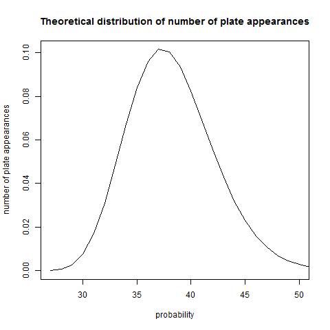
(Incidentally, if we set we get this model’s estimated probability of a perfect game. It’s (0.706)²⁷, which is about one per 12,000 team-games. There have been 21 perfect games since 1900 and about 360,000 total team-games since 1900, for one in 17,000 or so – roughly in the right neighborhood, at least, for such a crude model.)

It turns out that a baseball game is not quite long enough to get the distribution to totally equalize. Here’s a plot of the distribution of the number of plate appearances per game:

The distribution is not incredibly wide – the standard deivation is 3.99. Is this wide enough to get uniformity mod 9? Not quite. In the plot below, the red, green, and blue lines represent the probability of the game ending in the fourth, fifth, and sixth times through the order (28-36, 37-45, and 46-54 plate appearances, respectively), with the batter in the slot indicated on the x axis. The black line is the overall probability of ending on a given slot – the sum of the red, green, and blue lines, plus some other lines that are suppressed (games with 27 plate appearances, or 54 or more) that are graphically indistinguishable from zero.

The probability of the game ending with a batter in the kth slot in the order is given by the table below:

slot number	1	2	3	4	5	6	7	8	9
prrobability	.118	.114	.108	.104	.103	.106	.111	.116	.120

So the distribution is visibly not flat – but flat enough for Tango’s practical insight to make sense. Maybe moving someone up is expected to get them 17 extra plate appearances, or 19, instead of 18, depending on the slot. But the point still stands.  In practice the distribution of the final slot is probably even flatter than it appears here – the distribution of the number of plate appearances should be wider, since teams differ in skill, there are extra-inning games or games in which the home team doesn’t bat in the ninth, and so on.

Here’s a ten-minute video featuing Hannah Fry of UCL on the London riots of two summers ago. She’s a mathematician, and talks about the mathematics useful for understanding riots:
– the geography of rioting being like the geography of shopping – so certain parts of the city are more susceptible to rioting than others
– predator-prey interactions can br used to model the interaction between police and rioters
– the spread of the idea to riot is like the spread of an epidemic, and susceptibility to rioting seems to be connected to recent cuts in social services.

The original paper being described in this video is in Nature. I learned about it from FlowingData.

Greg Van Niel caught four foul balls at Sunday’s Cleveland Indians game.

ESPN reported that this is a one-in-a-trillion event – a number due to Ideal Seat, which I’ll take to mean that this guy had a one-in-a-trillion chance of catching four fouls. This is immediately suspicious to me. Total MLB attendance last year was about 75 million, so a one in a trillion event should happen once every thirteen thousand years. The fact that it happened, given that we’ve had way less than thirteen thousand years of baseball, is evidence that this computation was done incorrectly.

Somewhat surprisingly, given how small the number is, it actually seems to be an overestimate. I’ll assume that their numbers are correct: 30 balls enter the stands in an average game, and there are 30,000 fans at that game. Say I’m one of those fans. Let’s assume that all foul balls are hit independently, and that they’re equally likely to be caught by any person in the stands. The probability that exactly four balls will be hit to me are , where . This is about , or one in thirty trillion. (The probably that five or more balls will be hit to me is orders of magnitude lower than that.)

IdealSeat also claims that two fans caught two foul balls in the same game last year. I suspect that there’s some massive underreporting going on here, because the same analysis gives that the probability that I’ll get two balls is , which is about one in two million. So this should have happened 35 to 40 times last year – it’s just that most of the people who it happened to didn’t bother telling anybody! (Other than their friends, who probably didn’t believe them.)

What’s wrong with the one in a trillion, or one in thirty trillion, numbers?

• They assume that all foul balls are uniformly distributed over all the seats. This is patently untrue. Some seats by definition can’t receive a foul ball, because they’re in fair territory. Some seats, although they can theoretically receive a foul ball, just won’t. Ideal Seat has a heatmap of foul ball locations at Safeco Field in Seattle — basically the closer you are to home plate, the better your chances. Your chances of getting a foul ball drop off much faster with height than with horizontal distance. In addition, aisle seats are more likely to be the closest seat to where a ball lands than adjacent non-aisle seats.
• They assume that all foul ball locations are independent. I don’t know if there’s data on this, but batters have tendencies on where they hit balls in play; they should have tendencies on where they hit foul balls as well.
• They assume that a person can only get foul balls hit to their seat. This might be true in, say, San Francisco (where most games sell out), but it’s not true in Oakland (where there are plenty of empty seats). Van Niel’s section looks pretty full in the pictures, though. But Van Niel himself admits at least one of the balls wasn’t hit right to him.

All I can say for sure is that these drive the chances up – so the probability of catching four foul balls in a single game is probably a good deal higher than one in a trillion.

A visualization of normal versus fat-tailed distributions

Archimedes: Separating Myth from Science at the New York Times.

Daniel Walsh plays detective with rolling shutter photos: given a picture of a moving propeller, can you tell how fast it was moving?

Dave Richeson uses a kayak to measure the perimeter of a lake.

From Brain Facts, some visualizations of nonlinear systems.

A profile of Aaron Clauset’s research on power laws and terrorism.

Academic doesn’t have a PhD problem. It has an attitude problem.

Gil Kalai givces a solution to auction-based tic tac toe.

the Guardian has a video in which Paul Klemperer talks about geometry and the banking crisis. Surprisingly it’s tropical geometry to the rescue in resource allocation problems, as seen in this paper by Klemperer and Elizabeth Baldwin.

Brian Whitman tells us how music recommendation works and doesn’t work.

From yhat, handwritten digit recognition with node and python.

I asked about a month ago are Amazon rankings Zipfian?

Morris Rosenthal, a self-publishing author, has an interest in this subject for obvious reasons; he’s got some interesting-looking resutls for both paper books and e-books. Roughly speaking, yes; the most interesting thing I notice is that the slope of the rank vs. estimated sales curve (on a log-log scale) is higher both at the head (best-seller) and in the tail of the distribution compared to its bulk. What to make of this, I don’t know.

Chad Orzel, a physicist and author of How To Teach Physics to Your Dog took his own shot at this question a couple years ago.

David Eppstein asks: how many riffles does it take until all permutations are possible?

A riffle shuffle permutation, in the mathematics of shuffling cards, is a permutation of the cards that can be obtained by a single riffle shuffle — that is, you cut the deck into two packets and then interleave the packets. There are distinct riffle shuffles of n cards. For example, consider a five-card deck, which is initially in the order 1, 2, 3, 4, 5. Then a riffle shuffle consists of:

• cutting the deck in one of the six possible ways: 12345/ (no cut), 1234/5, 123/45, 12/345, 1/2345, /12345 (also no cut) where the slash represents the cut.
• riffling. For example look at 123/45. There are possible ways to make a permutation from this – we decide which two slots to put the 4 and the 5 in, and then everything else is forced. For example if we decide that 4 and 5 will go in the second and fourth positions, we must get 14253. In general if we have k cards in the left-hand pile and cards in the right-hand pile, we have $\latex n \choose k$ possible shuffles. Furthermore we can decompose any one of these permutations into two “rising sequences” in exactly one way, so it can come from exactly one cut — with a single exception. That exception is the identity permutation , which we can obtain from any of the n+1 possible cuts — so we must subtract n for the duplications. (If you put probabilities on this it becomes the Gilbert-Shannon-Reeds model.

Eppstein asks how many riffle shuffles it takes for each permutation to have nonzero probability. Since there are outcomes of a single riffle shuffle, in k iterations there are at most possible results. There will actually be less, because there are relations among the permutation subgroup generated by the riffle shuffles. (In less fancy language, there are sequences of different shuffles which give the same result. It’s the pedigree collapse of shuffling.)

Let’s replace this with to make the math easier. Now, there are permutations; this is greater than by a standard bound. So just in order to have possible sequences of shuffles of length k, we have to have , or, taking nth roots of both sides, . Taking base-2 logs, we get .

Eppstein gives a dynamical systems argument that you need at least $\lceil \log_2 n \rceil$ shuffles – and it turns out that that’s enough. This is in comparison to the classic result of Bayer and Diaconis, claiming that you need $3/2 \log_2 n$ shuffles to get a well-shuffled deck.