Error propagation for Atwood’s machine, by simulation

A few weeks ago I mentioned that the propagation of errors is a bit tricky. Say we want to predict the acceleration in an Atwood machine. The machine consists of a string extended over a pulley with masses at either end, of masses M and m, with M > m. The acceleration is given by

where g is the acceleration due to gravity, which we assume is known exactly. Let’s set g = 1, so we’ll have

We previously found by analytic methods that if and , then . But it’s instructive to do a simulation.

Specifically, fix some large . For , let be normally distributed with mean 100 and standard deviation 1; let be normally distributed with mean 50 and standard deviation 1; and let . Then the mean and standard deviation of the are estimates of the expected acceleration and its error.

This is very easy in R:


n = 10^4;
M = rnorm(n, 100, 1);
m = rnorm(n, 50, 1);
a = (M-m)/(M+m);


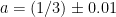
When I ran this code I got mean(a) = 0.3333875, sd(a) = 0.00993982. Furthermore, the computed values of a are roughly normally distributed, as shown by this histogram and Q-Q plot. (The line on the Q-Q plot passes through the point (0, mean(a)) and has slope sd(a).)

This works even if the errors are not normally distributed. For example, we can draw the simulated data from a uniform distribution with the given mean and standard deviation:


Mu = runif(n, 100-sqrt(3), 100+sqrt(3))
mu = runif(n, 50-sqrt(3), 50+sqrt(3))
au = (Mu-mu)/(Mu+mu)


I got mean(au) = 0.3332557 and sd(au) = 0.009936519. The distribution of the simulated results is a bit unusual-looking:

There’s also a way to compute an approximation to the error of the result using calculus, but simulation is cheap.