
I tried to Google this and couldn’t – how many people live in places where the polls close tonight at time X, for each possible value of X? You can easily find a map of closing times, for example at 270towin.com:
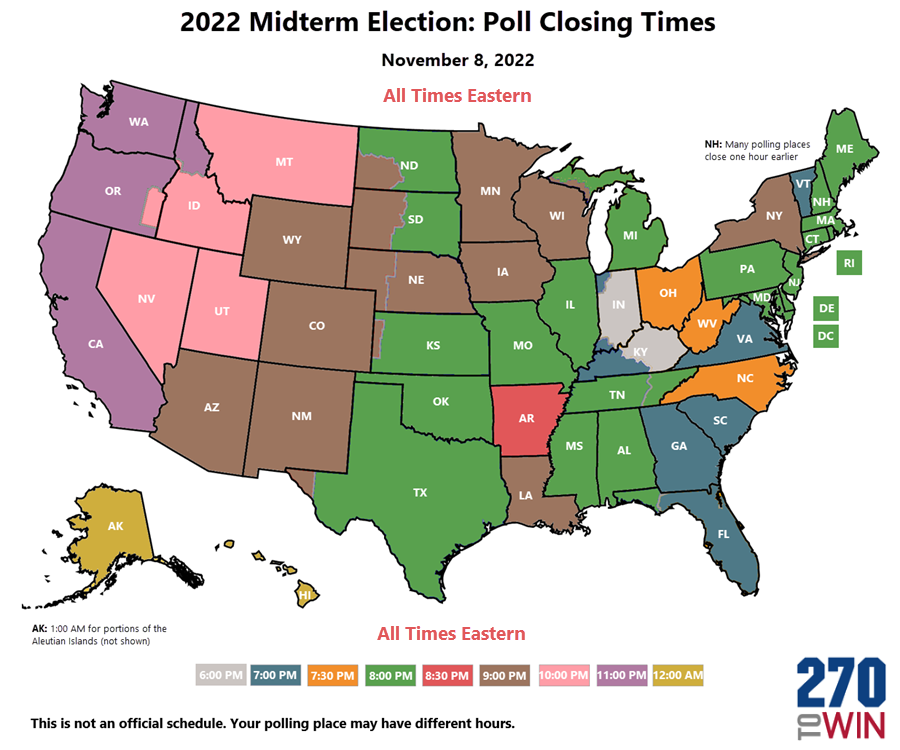
But how many people do each of those colors represent?
The Green Papers has a nice table of poll closing times. The wrinkle is that in a state with multiple time zones, there are two possibilities:- polls close at the same clock time across the state. For example, in Florida, polls close at 7:00 PM everywhere in the state… as we learned in 2000 when it was called for Democrats before polls in the Panhandle (the westernmost part of the state, the only part on Central time, and a heavily Republican area) had closed. This is the method in Alaska, Florida, Idaho, Kansas, Kentucky, Michigan, North Dakota, South Dakota, and Texas.
- polls close at the same real time across the state. This is what Nebraska does (8 Central / 7 Mountain) and Tennessee (8 Eastern / 7 Central).
As it turns out, in most places the polls close at 7 or 8 local time, and those represent about equal numbers of people. The exceptions are:
- Kentucky and Indiana (6 pm local)
- North Carolina, Ohio, West Virginia, and Arkansas: 7:30 pm local
- New York and North Dakota: 9 pm local. (Is there anything else New York and North Dakota have in common?)
The overall distribution is in the chart below.

And in Eastern-time terms, the distribution is:

Both of these charts and the underlying data are at this Google spreadsheet.
This should be familiar to people who make a habit of watching the election returns roll in… you get the first substantial votes at 7, a big chunk at 8, and they trickle in over the rest of the night. (In presidential years the 11:00 chunk isn’t as interesting as you’d expect from its volume – the only polls closing at 11 are California, Oregon, Washington, and small portions of North Dakota and Idaho, and if any of those states are competitive the election as a whole is not.)
Too small to show on the chart is the polls that close at 1 AM. Those are the polls that close at 8 PM (Hawaii-)Aleutian time (UTC-10, five hours behind Eastern time), in that part of the Aleutian Islands of Alaska west of 169° 30′ W longitude. In terms of populated places it looks like this is a really long-winded way of saying Adak. Adak has 326 people. The biggest settlement in the Aleutians, Unalaska, is only at 166° 32′ W and is therefore in UTC-9, “Alaska time”. Brian Brettschneider, Alaska-based climatologist, called out Adak in 2016:
https://platform.twitter.com/widgets.jsThe last voting location to close in the U.S. is at the Adak, Alaska, school. #akelect pic.twitter.com/a7ZyXa1c9R
— Brian Brettschneider (@Climatologist49) November 8, 2016
and at least a cursory look at a list of Alaska polling places suggests there are two in the Aleutians, “Aleutians No. 1” in Adak and “Aleutians No. 2” in Unalaska. It seems quite reasonable that there is only one polling place, the one in Adak, that closes at 1 AM Eastern. This oddity has been mentioned before, in 2012 and 2016, in both cases by local sources. In 2016 five people voted after 8 PM Alaska / 7 PM Aleutian (midnight Eastern).
Not that anything will be called in Alaska when the polls close… Alaska uses ranked-choice voting, so it’ll take a while to count the votes anyway.


 win with the target sums
  if and only if the dice values
  win with the target sums
  .
. rows, one for each of the 1296 possible dice rolls and 330 choices of targets.
  set if
  is one of the targets;
  set if
  is one of the pairwise sums. Then
  and
and  . And
. And  . Since it’s greater than zero, that counts as a win.

 . So we need to find positive integers x, y, z such that x + y + z = 100 and

 . The three big factors – the two 7s and the 11 – look like they’ll be worrisome. So let’s spread them out: let x and y both be multiples of 7, and let z be a multiple of 11. To get them to add up to 100, we need to find a multiple of 7 and a multiple of 11 that add up to 100; it’s easy to find 44 and 56. So z = 44.
  , so x and y must be 21 and 35.
  will have many factors, and many ways to be written as a product of three integers, making it more likely that one of those will have the right sum.
 .
.  , and the probabilities of getting n+2, n+3, …, 2n are
  – generalizing the well-known triangular distribution. The probability that you and your friend both roll 2, then, is

 , so we should get a result of order 1/n. We can peservere and do the algebra and we get
 . He writes that “the percentage chance of a match score falls off a lot slower than I would have predicted.”
 are possible with any appreciable frequency. There are on the order of a few square roots of k of these, so the answer should be
  for some
  . Like Berry, I am too lazy to find the constant
  .
. , by approximating both sums as normal and applying the central limit theorem. This is about
  . If we bear in mind that the variance of a single roll of an n-sided die is
  , then we get
  for rolling k n-sided dice.
 . This reduces to 1/n, the correct answer, if you let
  and ignore the -1.
 , so clearly
  . (All logarithms in this post are to base 10.) Can we approximate the logs of any other primes this way?
 .
. 
 . And of course we have
  , so this relation becomes
 .
. and $\log 4374 \approx \log 4375$, namely

 .
. .
. (a fundamental fact of musical temperament).
  right away,
  , and then
  so
so  . This is essentially I. J. Good’s
  , the fact on which our usual musical tuning system is based:
  , and a bit less accurately
  . (Musically these are the facts that the perfect fifth, major third, and minor seventh are the ratios 3/2, 5/4, and 7/4.).
  , which gives
  . This is a less good approximation than those of
  and
and  , just as the seventh harmonic isn’t really a note in the equal-tempered scale –