So everyone knows that correlation coefficients are between  and
and  . The (Pearson) correlation coefficient of
  and
and  is given by
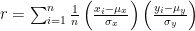
where  are the means of the
  and
and  , and
, and  are their (population) standard deviations. Alternatively, after some rearrangement this is

which is more convenient for calculation, but in my opinion less convenient for understanding. The correlation coefficient will be positive when  and
and  usually have the same sign — meaning that larger than average values of
  go with larger than average values of
  — and negative when the signs tend to be mismatched.
But why should this be between and ? That’s not at all obvious from just looking at the formula. From a very informal survey of the textbooks lying around my office, if a text defines random variables then it gives a proof in terms of them. For example, Pitman, Probability, p. 433, has the following proof (paraphrased): Say  and
and  are random variables and
  ,
,  are their standardizations. First define correlation for random variables as
  . Simple properties of random variables give
  . Then observe that
  and look at

and rearrange to get that  . Similarly looking at
  gives
gives  . Finally, the correlation of a data set is just the correlation of the corresponding random variables.
This is all well and good if you’re introducing random variables. But one of the texts I’m teaching from this semester (Freedman, Pisani, and Purves, Statistics) doesn’t, and the other (Moore, McCabe, and Craig, Introduction to the Practice of Statistics) introduces the correlation for sets of bivariate data before it introduces random variables. These texts just baldly state that  is between and always — but of course some students ask why.
The inequality we’re talking about is an inequality involving sums of products: it’s really  . And that reminded me of the Cauchy-Schwarz inequality — but how to prove Cauchy-Schwarz for people who haven’t taken linear algebra? Wikipedia comes to the rescue. We only need the special case in
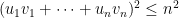
  , in which case Cauchy-Schwarz reduces to

for any real numbers  . And the proof at Wikipedia is simple: look at the polynomial (in
  )
)

This is a quadratic. As a sum of squares of real numbers it’s nonnegative, so it has at most one real root. So its discriminant is nonpositive. But we can write it as

and so its discriminant is

and this being nonpositive is exactly the form of Cauchy-Schwarz we needed.
To show that this implies the correlation coefficient being in ![[-1, 1]](https://s0.wp.com/latex.php?latex=%5B-1%2C+1%5D&bg=ffffff&fg=000000&s=0&c=20201002) : let’s say we have the data
: let’s say we have the data  and we’d like to compute the correlation between the and the
  . The correlation doesn’t change under linear transformations of the data. So let $u_i$ be standardizations of the $x_i$ and let $v_j$ be standardizations of the $y_j$. Then we want the correlation in
  . But this is just

By Cauchy-Schwarz we know that

and the right-hand side is  , since
  is the standard deviation of the
  , and similarly for the other factor. Therefore
and dividing through by gives that the square of the correlation is bounded above by $1$, which is what we wanted.
So now I have something to tell my students other than “you need to know about random variables”, which is always nice. Not that it would kill them to know about random variables. But I’m finding that intro stat courses are full of these black boxes that some students will accept and some want to open.
 rotations, where
  , then leaves tend to be arranged in such a way that they don’t cover each other up. I actually hadn’t known that Lucas numbers show up in phyllotaxis as well — the relevant angle is
  of a circle. And the whole thing comes from the mutual repulsion of the growing leaves.