I’m reading John R. Taylor’s textbook An Introduction to Error Analysis: The study of uncertainties in physical measurements. This is meant for people taking introductory physics lab classes, but it never hurts to revisit these things. I actually double-majored in math and chemistry in college. It’s fun watching the contortions that chemists go to to avoid math.
Anyway, measurements come with uncertainities: that is, they have the form 


– that is, the variances attached to the measurements add. Similarly, for differences,
. For example,
and
. Note that the error for the sum and the difference are the same – but for the difference, the error is relatively much bigger.
- To find
, start by finding the fractional uncertainties
and
. Then the squares of the fractional uncertainties add: the fractional uncertainty of the product is
. The same fractional uncertainty holds for quotients. For example, the fractional uncertainty in
is
, and that in
is
. So the fractional uncertainty in their product is $\sqrt{(0.133)^2 + (0.15)^2 = 0.201$. Thus we have for the product
and for the quotient
.
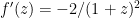
- Perhaps one learns rules for dealing with powers, logarithms, and the like. These are all easily derived from the rule
.
For example,


In this case, the fractional uncertainty becomes the absolute uncertainty in the logarithm. If we know a number to within ten percent, we know its log to within 0.1 unit.

But implicit in the rules for sums, differences, products, and quotients is the idea that the errors 


So what can we do? In this particular case it’s not hard to rewrite as
where 


Alternatively, we think that 
![0.5 \pm 0.011 = [0.489, 0.511]](https://s0.wp.com/latex.php?latex=0.5+%5Cpm+0.011+%3D+%5B0.489%2C+0.511%5D&bg=ffffff&fg=000000&s=0&c=20201002)
But we are not guaranteed that our rewriting trick will always work. What else can we do? I’ll address that in a future post.

Allow me to toot my horn.
I taught physical chemistry laboratory, before I retired. I’d try to get my students to do an error estimate on their measurements and on the computed results. It proved to be hard to get them to make reasonable estimates of the errors in measurements. The best method of propagation to an over-all estimate of the error in the final computed results seemed to me to be the following. Compute the result, recompute with one input measurement incremented by the estimate of its error, take the difference to get the contribution of that input error. Repeat for each input piece of data. Square the separate computed errors, add the squares, take the square root. (Easy enough to do with a good spread sheet program.) That gives a pretty good estimate of the final error in the computed result, if the estimates of the errors in the input measurements are good. Of course, that was the problem. Read a thermometer with one degree divisions marked on the stem at intervals of about 4mm? Then obviously the error is one degree. (Never mind that one can estimate the temperature to a tenth of a degree with perhaps a one sigma error of one tenth of a degree.) The advantage of this method over what is being described in the part of Taylor you are presenting is that it is justifiable for pretty much all sources of error, whether related to the output linearly, or exponentially, or in some complex way that is not easy to describe in the elementary formulas. The seemingly simple experimental determination of the heat capacity ratio of an ideal gas by the adiabatic expansion method is an example of such complexity, as the measured atmospheric pressure is used several times in the calculation.
As an excellent short introduction and with a very good section on error propagation (perhaps as a suggested textbook) you might find Hughe’s and Hase’s – Measurements and Their Uncertainties interesting as well.