On propagation of errors

I’m reading John R. Taylor’s textbook An Introduction to Error Analysis: The study of uncertainties in physical measurements. This is meant for people taking introductory physics lab classes, but it never hurts to revisit these things. I actually double-majored in math and chemistry in college. It’s fun watching the contortions that chemists go to to avoid math.

Anyway, measurements come with uncertainities: that is, they have the form $x \pm \delta_x$ , where $x$ is our best estimate of the quantity and $\delta_x$ is an estimate of the uncertainty. (We can think of this as being roughly the standard deviation of the distribution from which $x$ is drawn.) In these intro lab classes one quickly learns some rules for manipulating these uncertainties. These can be thought of as defining arithmetic on intervals; however this isn’t the usual interval arithmetic but actually an abbreviation of arithmetic on probability distributions.

$(x \pm \delta_x) + (y \pm \delta_y) = (x+y) \pm (\sqrt{\delta_x^2 + \delta_y^2})$ – that is, the variances attached to the measurements add. Similarly, for differences, $(x \pm \delta_x) - (y \pm \delta_y) = (x-y) \pm (\sqrt{\delta_x^2 + \delta_y^2})$ . For example, $(30 \pm 4) + (20 \pm 3) = (50 \pm 5)$ and $(30 \pm 4) - (20 \pm 3) = (10 \pm 5)$ . Note that the error for the sum and the difference are the same – but for the difference, the error is relatively much bigger.
To find $(x \pm \delta x) \times (y \pm \delta_y)$ , start by finding the fractional uncertainties $\delta_x/x$ and $\delta_y/y$ . Then the squares of the fractional uncertainties add: the fractional uncertainty of the product is $\sqrt{(\delta_x/x)^2 + (\delta_y/y)^2}$ . The same fractional uncertainty holds for quotients. For example, the fractional uncertainty in $30 \pm 4$ is $4/30 \approx 0.133$ , and that in $20 \pm 3$ is $3/20 = 0.15$ . So the fractional uncertainty in their product is $\sqrt{(0.133)^2 + (0.15)^2 = 0.201$. Thus we have for the product $600 \pm 120$ and for the quotient $1.5 \pm 0.3$ .
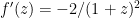
Perhaps one learns rules for dealing with powers, logarithms, and the like. These are all easily derived from the rule $f(x \pm \delta x) = f(x) \pm |f\prime(x) \delta x|$ .

For example,
$(30 \pm 4)^2 = 30^2 \pm |(2)(30)(4)| = 900 \pm 240$ – in fact, when taking nth powers, the fractional uncertainty is raised to the $n$ power. Similarly,
$\log (30 \pm 4) = \log 30 \pm |(1/30) (4)| = 1.48 \pm 0.13.$
In this case, the fractional uncertainty becomes the absolute uncertainty in the logarithm. If we know a number to within ten percent, we know its log to within 0.1 unit.

But implicit in the rules for sums, differences, products, and quotients is the idea that the errors $\delta x, \delta y$ in the measurements of $x, y$ are independent! So these rules can’t be used if there’s correlation between the errors. More simply, they can’t be used if the quantity that you’re interested in is a function of many variables, some of which occur more than once. Consider for example the Atwood machine, as Taylor does in his problem 3.47. This consists of two objects, of masses $M$ and $m$ with $M > m$ ; the larger mass accelerates downward, with acceleration $a = g(M-m)/(M+m)$ . Here $g$ is the acceleration due to gravity. We assume this is known exactly. So there may be correlation between the numerator and the denominator.

So what can we do? In this particular case it’s not hard to rewrite as
$a = g {1-(m/M) \over 1+(m/M)} = g f(m/M)$
where $f(z) = (1-z)/(1+z)$ , and use the rules that I’ve already discussed. (But it may be hard to see that this is worth doing!) For example (I’m taking these numbers from Taylor) say $M = 100 \pm 1, m = 50 \pm 1$ . Then the fractional uncertainty in the quotient $M/m$ is $\sqrt{(0.01)^2 + (0.02)^2} \approx 0.022$ , and we get $M/m = 0.5 \pm 0.011$ . Then $f^\prime(z) = -2/(1+z)^2$ , so $f^\prime(1/2) = -8/9$ , and thus we have $f(M/m) = f(1/2) \pm (0.011)(8/9) = (1/3) \pm 0.01$ .

Alternatively, we think that $m/M$ is likely to lie in the interval $0.5 \pm 0.011 = [0.489, 0.511]$ ; then f(0.489) = 0.343 and f(0.511) = 0.324, so we figure that f(m/M) is likely to lie in the interval [0.324, 0.343].

But we are not guaranteed that our rewriting trick will always work. What else can we do? I’ll address that in a future post.

Weekly links for March 25

You can buy anacrylic Frabjous kit or get your very own cardboard Frabjous.

Online matchmaking is not so great, because it leads you to focus on things that are easily measured.

The hard way to solve the 8809=6 puzzle (with regression!); I solved it here. (I actually thought about using regression. But I did not.)

Statistics project ideas for students.

Cheating on homework in a graduate course is staggeringly dumb. This post and its comments are not, and attempt to answer the question: what’s the point of homework in math classes? (If I were a better blogger, or if I were not seeing an amazing lady like one of the commenters was, I’d have an answer of my own.)

The anachronism machine: the language of Downtown Abbey. (The typo is deliberate; I don’t watch the show.)

You can look at brains and see math anxiety.

A working scientific calculator, built in Minecraft. (via metafilter)

David Spiegelhalter on What does a 13% increased risk of death mean??

Cultural ontogeny recapitulates phylogeny

The MIT course 6.042: Mathematics for Computer Science has a textbook in progress by Eric Lehman (Google), F. Thomson Leighton (MIT math/CS, Akamai), Albert Meyer (MIT EECS, MIT CSAIL); various versions of it in various stages of completion are available from their course web page. (via Hacker News.)

Jordan Ellenberg at Slate: Six Degrees of Innovation: What Broadway musicals tell us about creativity.

From stackoverflow, How do I find Waldo with Mathematica?

A geographical existence proof

If you spend time in the Mission in San Francisco, you think of Mission Street and Van Ness Avenue as both running north-south, with Mission parallel to and slightly to the west of Van Ness.

But north of there, Mission is one of the major streets downtown, and Van Ness runs through neighborhoods to the west of downtown. That is, Mission is now east of Van Ness.

Therefore, if you assume that each street exists only in one piece, they must cross each other. A sketch of a proof, which works because the streets aren’t too curvy: any line of latitude within the part of the city in question intersects each of Van Ness and Mission, exactly once. Take the difference between the longitude (west of Greenwich, because why not?) at which that line intersects Van Ness and the longitude at which it intersects Mission. At the latitude of, say, 24th Street, this is negative (Van Ness is east of Mission, so has smaller numerical longitude) and at the latitude of, say, Geary, this is positive. By the intermediate value theorem it must be zero at some point, the latitude of the intersection.

(Inspired by being caught in a traffic jam a few days ago, near the intersection of Van Ness and Mission, which I had previously not recognized existed, despite being familiar with both streets on both sides of the intersection.)

Comments on Johnson’s predictions of Olympic medal counts

Daniel Johnson of Colorado College predicts Olympic medal counts.

The model is based only on non-athletic factors. Johnson’s semi-technical summary of the model gives the formula used. The variables used in the prediction are as follows:

the total number of medals available
per capita income
population
whether the Olympics are being held in that country this year, or in the near future or near past, or in a neighboring nation
a “nation-specific effect”

I’m not entirely sure what the “nation-specific effect” means, but I suspect it’s an adjustment for countries that consistently overperform or underperform the targets given by the rest of the model. I remember hearing in 2008 that it was quite strange that India, for example, did so poorly at the Olympics. (The explanation I heard a lot was that the Olympics don’t have cricket.) Australia, on the other hand, consistenly punches above its weight.

A working paper from 2002 suggests that previous iterations of the model also had climate-related variables; the press release says that it doesn’t any more, as those no longer seem to be significant. Presumably they are in the Winter Games and we’ll see them again in 2014.

For 2012, the predicted leaders in gold medals are the USA, China, Russia, Great Britain, and Germany; the predicted leaders in overall medals are the same, with Great Britain (the host country) and Germany reversed.

But is this overkill? Roger Pielke points out at freakonomics and at his own blog that the “naive” prediction that a country will do as well this year as it did four years ago has smaller errors than Johnson’s model. Johnson replies in a comment to Pielke that his model isn’t intended for predicting what each country will do, it’s intended to show which factors are important for Olympic success. In other words, he’s interested in the coefficients of his model and how they change over time, not what you get when you plug in values for any specific country.

(via Freakonomics and Forbes. more information from Johnson’s web site.)

Absence of evidence is not evidence of absence, but it helps.

A long time ago in a city far far away I was a grad student.

Now here at Berkeley it is qualifying exam season, and the following exchange took place in an elevator:

Professor X: “I was at A’s a qualifying exam today.”
Grad student Y: “How did A do?”
Professor X: “He was great!”

Of course, X wouldn’t have said that A did well if A had done poorly. But he probably also wouldn’t have said that A did poorly; instead he would have hemmed and hawed and avoiding saying anything at all. And that would have told Y what she wanted to know.

Similarly, I remember that when I was in grad school, the information that someone had passed their qualifying exam spread quite quickly among the students, whereas the information that someone failed spread less quickly. The reason for this is simple: passing is happy news, so the person who passed and their friends will tell everyone. But failing is sad news, so you can really only find out if someone failed by specifically asking them.

So assume that rumors spread according to a logistic model, and furthermore that the information of a success spreads twice as quickly (for small populations) as the information of a failure. That is, the proportion of the population that knows that person X succeeded at time $t$ after their exam is

$P_1(t) = {1 \over 1+C_1 e^{-t}}$

and the proportion that knows that person Y failed at time $t$ after their exam is

$P_2(t) = {1 \over 1+C_2 e^{-t/2}}$

for some different constant $C_2$ . Furthermore $P_1(0) = P_2(0) = 1/(n+1)$ , where $n+1$ is the number of students; solving gives $C_1 = C_2 = n$ .

So say it’s time t, and you haven’t heard if the person who had their exam at time 0 passed or not. Then by Bayes’ theorem, the odds in favor of their passing are that they’ve passed is

$O(pass|N) = O(pass) {P(N|pass) \over P(N|fail)}$

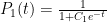
where $O(\cdot)$ denotes the odds of $\cdot$ $N$ denotes the event of not having heard yet. Typical pass rates at the time I was there were perhaps 3 out of 4, so $O(pass) \approx 3$ . The conditional odds are therefore

$O(pass|N) = 3 {P(N|pass) \over P(N|fail)}.$

But $P(N|pass) = 1-P_1(t)$ and $P(N|fail) = 1-P_2(t)$ . So, after some algebra,

${P(N|pass) \over P(N|fail)} = {{1 \over n} e^{t/2} + 1 \over {1 \over n} e^t + 1}$

and indeed this decays (exponentially fast!) as $t \to \infty$ . So the longer you go without hearing the news of someone’s exam outcome, the more likely it is that it’s bad news.

Of course reality is more complicated. This doesn’t take into account the structure of the social network. For example, for any given person there’s probably a ring of people at a certain social distance who would hear very quickly if they passed but not if they failed. If you know that you are in that relationship to a person, you can probably guess with pretty near certainty that they failed if you don’t hear right away.

A puzzle from James Tanton

James Tanton asks in a series of tweets (which I’ve modified slightly): Write 20 numbers. Erase any two, $a$ and $b$ , and replace with $f(a,b)$ , where some possible choices of $f(a,b)$ are:

$f_1(a,b) = a+b+ab$ (here)
$f_2(a,b) = \sqrt{a^2+b^2}$ (here)
$f_3(a,b) = ab/(a+b)$ (here)
$f_4(a,b) = \log(e^a+e^b)$ (here)

Repeat 19 times, until you get a single number. The final result will be independent of the choices of pairs made. Why?

For example, consider $f(a,b) = a+b+ab$ . And say we start with the numbers 2, 3, 6, 7. Then we could choose to do the replacement as follows. In each case the two bolded numbers are replaced by one.

2, 3, 6, 7 becomes 3, 7, 20
3, 7, 20 becomes 7, 83
7, 83 becomes 671

and so we’re left with 671. Or we could have

2, 3, 6, 7 becomes 2, 7, 27
2, 7, 27 becomes 23, 27
23, 27 becomes 671

and again we’re left with 671. What’s going on here? It’s not immediately apparent, but if you try this starting with lots of small integers, you often get results which are one less than some number with many small factors — in this case, 672. And in fact $672 = (3)(4)(7)(8)$ , which we can rewrite as

$671 + 1 = (2+1)(3+1)(6+1)(7+1).$

We can think of the whole process, starting with $x_1, x_2, \ldots, x_n$ , as computing the product $(x_1+1) (x_2+1) \cdots (x_n+1)$ by combining two factors at a time; of course the order doesn’t matter.

Similarly with the function $f_2$ , if we start with $x_1, x_2, \ldots, x_n$ we end up with $\sqrt{x_1^2 + \cdots + x_n^2}$ . With $f_4$ , we get $\log \left( e^{x_1} + e^{x_2} + \cdots + e^{x_n} \right)$ . The result with $f_3$ is a little harder to see but if we start with $x_1, \ldots, x_n$ we eventually get $1/(x_1^{-1} + \cdots + x_n^{-1})$ . This is a bit easier to see if we realize that $f_3(a,b) = (1/a + 1/b)^{-1}$ ; therefore applying $f_3$ conserves the sum of the reciprocals.

What others are there? Of course there are trivial examples like $f(a,b) = a+b$ and $f(a,b) = ab$ ; iterating these functions will just give the sum or the product of the original numbers. But what other nontrivial examples are there? Can you say what all of them are?

A third of my life

I’m 28 years old. A perfect age! (Don’t wish me a happy birthday, I’ve been 28 for a few months.)

Recently it occurred to me that I’ve lived a third of my life, at least if you believe the classic biography of Diophantus:

‘Here lies Diophantus,’ the wonder behold.
Through art algebraic, the stone tells how old:
‘God gave him his boyhood one-sixth of his life,
One twelfth more as youth while whiskers grew rife;
And then yet one-seventh ere marriage begun;
In five years there came a bouncing new son.
Alas, the dear child of master and sage
After attaining half the measure of his father’s life chill fate took him. After consoling his fate by the science of numbers for four years, he ended his life.’

(translation from Wikipedia)

I’m pretentious enough to quote this in Latin, except that I don’t know Latin. If you are pretentious enough to know Latin (and I think I have at least one reader who is), go to the Wikipedia article for the original.

But there are other classical amounts of time that are cited as the typical lifespan: “three score years and ten” Psalm 90:10 is the most frequently mentioned. Genesis 6:3 suggests that the maximum human liefspan is 120 years. My father says he’ll live until 100 (I think he started saying this in his forties, so he could convince himself that he wasn’t middle-aged yet).

So what proportion of my life have I lived? Or, because you don’t care about me, what proportion of one’s life has one lived at age X? We can’t just divide by the life expectancy. Let’s say life expectancy is 70; then I’d have lived two-fifths of my life by now. But that means that when I am 70, I will have lived my entire life. And when I’m 77, I will have lived 110% of my life! Clearly the proportion of my life that I’ve lived, at 28, is 28 divided by the expected age at which a 28-year-old dies. A quick look at a life table says that the “expectation of life at age [28]” is 50.8 — so a typical 28-year-old should expect to live to 28 + 50.8 = 77.8. Therefore I have lived 28/78.8 of my life, or about 35.5 percent. The life expectancy at birth, according to the same table, is 77.4, and 28/77.4 is about 36.2 percent. I just got 0.7 percent of my life back by doing this calculation! But I’ve probably spent more than 0.7 percent of my life learning how to do such calculations.

Weekly links for March 18

Vladimir Bulatov, Conformal models of hyperbolic geometry.

The chance shirt machine (auf Deutsch).

The personal analytics of [Stephen Wolfram’s] life.

Wooden stick models of Archimedean solids.

Laura McLay, The conditional probability of being struck by lightning, parts one and two.

Jordan Ellenberg’s review of William Cook’s In pursuit of the traveling salesman: mathematics at the limits of computation.

Modern nomograms for sale, via Dead Reckonings: Lost Art in the Mathematical Sciences.

The Poisson process of e-mail.

Foursquare asks: What neighborhood is the ‘East Village’ of San Francisco?, based on what type of establishments people check into in various neighborhoods.

Isarithmic maps of public opinion data.

Duels, truels, and game theory gunslinger rules, by David Barash, author of The Survival Game: How Game Theory Explains the Biology of Cooperation and Competition (which I have not read).

Brad Efron’s notes on large-scale simultaneous inference.

Galperin’s billiard method of computing pi, from Calculus VII.

Spiked Math IQ Test. I got a zero. Perhaps knowing this will help you get better than zero.

Taking PhD comics too literally

March 14 PhD comics includes a plot. The x-axis is “time spent staring at your computer” and the y-axis is “probability you’ll come up with a brilliant idea”. The graph is a horizontal line.

This has two possible interpretations:

the intended one: at least at the time depicted in the comic, no ideas come. this corresponds to interpreting the y-axis as the cumulative probability that an idea will come by time x.
the hopeful one: let’s say I stare at my computer for 24 hours straight, starting now. The probability that I come up with a brilliant idea between 11:00 AM and 11:01 AM, say, is the same as the probability that I come up with a brilliant idea between 11:00 PM and 11:01 PM. In other words, brilliant-idea-having is a Poisson process. But then if I wait long enough, I should almost certainly come up with a good idea. This corresponds to interpreting the y-axis as the rate of a Poisson process at time x.

The truth is probably somewhere in between: 40 hours a week is as productive as 55. And Cham, we’re meant to understand, is depicting that part after 40 hours in a week where the brain just won’t get more done.

My name is supervocalic

So it was pointed out to me yesterday that my name (“Michael Lugo”) has each of the five vowels (a, e, i, o, u) exactly once. Such a word is called supervocalic.
What are the chances of that?

A quick calculation: assume that letters have the frequencies given in the Wikipedia article for English. In particular the frequencies of A, E, I, O, and U are 8.167%, 12.702%, 6.966%, 7.507%, 2.758%. The frequency of all other letters combined is 61.900%; call this q. Call the product of these c; the value of c is about $1.50 \times 10^{-6}$ .

Now assume that names are created by picking letters independently at random. To construct a string in which each vowel appears exactly once, we must:

decide where the vowels will appear. We can do this in $n(n-1)(n-2)(n-3)(n-4) = n!/(n-5)!$ ways; here order matters.
put A, E, I, O, U in those five pre-chosen positions, and consonants in the others; the probability of this is $C q^{n-5}$ .

So a string of length n has probability ${n! \over (n-5)!} C q^{n-5}$ of having each vowel occur exactly once. For $n = 6, 7, \ldots, 20$ I give those probabilities in the following table:

6	7	8	9	10	11	12	13	14	15	16	17	18	19	20
0.0007	0.0014	0.0024	0.0033	0.0041	0.0047	0.0050	0.0050	0.0048	0.0045	0.0040	0.0035	0.0030	0.0025	0.0021

For example, a name of length 11 (like mine) has probability about 0.0047 of containing each vowel exactly once. The string length which is most likely to be supervocalic is 13; that makes sense, as a typical string is thirty-eight percent vowels, and five is about thirty-eight percent of thirteen. It’s hard to go much further with this, though, because I don’t have the distribution of lengths of names. But whatever the distribution of name lengths, the proportion of supervocalic names is bounded above by one in two hundred. Special, but not that special. (My instinct is that supervocalic names are probably a bit more likely than this, because the distribution of the number of vowels in a name of length $n$ is probably more tightly concentrated than a binomial.)

Ken Jennings has a list of sets that contain exactly one such word, many of which contain less than a couple hundred elements, but it’s hard to say what that means in this context. For more words with this property, see the message boards; in particular there are some nine-letter examples. Getting much shorter than that seems to interfere with euphony, which my model doesn’t take into account. There have been 250 major league baseball players who have each vowel at least once; many have each vowel exactly once. Many of them are named Charlie; few, it seems, are named Michael, because your typical baseball player is more likely to go by Mike.